2. Fitting SEDs with a Custom Model

This tutorial will walk you through customizing the B5 model and fitting the same AT2022cmc data as the first tutorial.

# imports

import numpy as np
import pandas as pd
import matplotlib.pyplot as plt
import syncfit

2.1. Reading in the Data

This is the same as the first tutorial, it is just here as a refresher.

# read in the data
cmc = pd.read_csv('AT2022cmc_Andreoni2022.txt')
cmc

	facility	date	dt	nu	F_nu	F_err	upperlimit
0	NOEMA	2022-03-24 22:14	41.48	86.0	3914	30	True
1	NOEMA	2022-03-24 22:14	41.48	102.0	3609	34	False
2	NOEMA	2022-03-25 00:45	41.58	136.0	3045	41	False
3	NOEMA	2022-03-25 00:45	41.58	152.0	2750	51	False
4	VLA	2022-03-31 04:08	47.73	31.4	2130	30	False
5	VLA	2022-03-31 04:08	47.73	33.5	2260	30	False
6	VLA	2022-03-31 04:08	47.73	35.6	2350	40	False
7	VLA	2022-03-31 04:08	47.73	37.5	2360	40	True
8	VLA	2022-03-31 04:13	47.73	8.5	270	12	False
9	VLA	2022-03-31 04:13	47.73	9.5	336	11	False
10	VLA	2022-03-31 04:13	47.73	10.5	385	12	False
11	VLA	2022-03-31 04:13	47.73	11.5	438	14	False
12	VLA	2022-03-31 04:23	47.74	12.8	583	12	False
13	VLA	2022-03-31 04:23	47.74	14.3	724	12	False
14	VLA	2022-03-31 04:23	47.74	15.9	801	14	True
15	VLA	2022-03-31 04:23	47.74	17.4	935	15	False

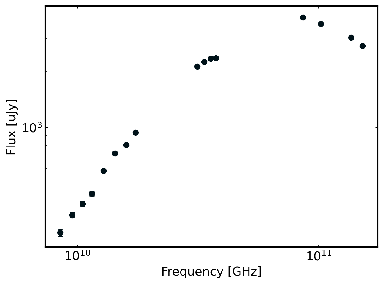
# now plot the SED
fig, ax = plt.subplots(1)

ax.errorbar(cmc.nu*1e9, cmc.F_nu, yerr=cmc.F_err, fmt='o')
ax.set_xscale('log')
ax.set_yscale('log')

ax.set_xlabel('Frequency [GHz]')
ax.set_ylabel('Flux [uJy]')

Text(0, 0.5, 'Flux [uJy]')

2.2. Fitting the Data

Now that we have the AT2022cmc data read in, we can fit it using syncfit. Let’s first just use the default B5 model like we did in the first tutorial.

# the initial guesses
theta_init = [
    3, # p-value guess
    1, # initial log_F_nu guess
    10, # initial nu_a guess, this is all we need for B5!
]

# the number of walkers
# 32 is usually fine, more makes it slower!
nwalkers = 32

# now define the number of iterations
# something small for now to make it fast,
# usually ~2000 gives a converging chaing
niter = 500

# now we can fit the data
sampler = syncfit.do_emcee(
    theta_init = theta_init,
    nu = cmc.nu,
    F_muJy = cmc.F_nu,
    F_error = cmc.F_err,
    model = syncfit.models.B5, # get the model from syncfit
    niter = niter,
    nwalkers = nwalkers
)

# Then let's just check how the fit looks
syncfit.analysis.plot_best_fit(
    model = syncfit.models.B5,
    sampler = sampler,

    # be careful with units for the data
    # the frequency must be in GHz space
    # and the flux densities must be in mJy space
    nu = cmc.nu*1e9,
    F = cmc.F_nu*1e-3
)

# print out the constraints we get
labels = syncfit.models.B5.get_labels()
constraints = syncfit.analysis.get_bounds(sampler, labels, toprint=True)

100%|███████████████████████████████████████████████████████████████████████████████| 500/500 [00:00<00:00, 2602.04it/s]

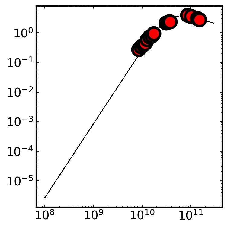
\mathrm{p} = 2.01e+00_{-0.005}^{0.487}
\mathrm{log F_v} = 7.87e-01_{-0.119}^{0.053}
\mathrm{log nu_a} = 1.05e+01_{-1.051}^{0.007}

Which has a pretty good looking fit! But, let’s see if we can make it better by customizing the B5 model a little more! For this tutorial, we are going to modify the prior function, called lnprior, but some other methods that can be customized are SED (the model itself) and loglik (the likelihood function which, by default, is just gaussian).

To do this, we use the decorator @syncfit.models.B5.override. All of the models, including the generic SyncfitModel model, have this override decorator which allows you to customize that specific method of the model class. If you want to use the generic SyncfitModel instead of one of the other builtin models please note that you will need to define lnprior, SED, and get_labels using this decorator.

@syncfit.models.B5.override
def lnprior(theta, p=None, **kwargs):
    '''
    Our customized lnprior function. This needs the arguments
    that it has and no more or less! Otherwise it won't work
    when we actually try to run the MCMC.
    '''

    # All of this is copied from the source code and is fine to leave
    # since it is just unpacking the theta value
    if p is None:
        p, log_F_nu, log_nu_a= theta
    else:
        log_F_nu, log_nu_a = theta

    # However, here we want to change things to narrow the
    # priors on all three parameters
    if 2.9 < p < 3.1 and -1 < log_F_nu < 1 and 9 < log_nu_a < 11:
        return 0.0

    else:
        return -np.inf

In this case, since we’ve just overwritten a method of the B5 model class directly, we can just pass in the B5 model again.

# now we can fit the data
sampler = syncfit.do_emcee(
    theta_init = theta_init,
    nu = cmc.nu,
    F_muJy = cmc.F_nu,
    F_error = cmc.F_err,
    model = syncfit.models.B5, # use the same model here!
    niter = niter,
    nwalkers = nwalkers
)

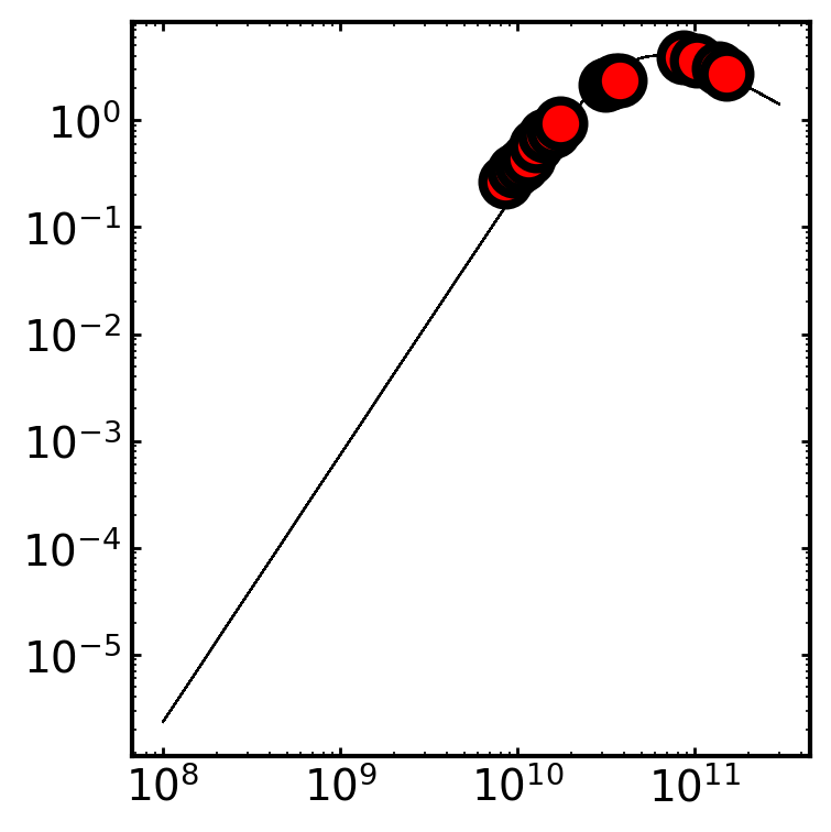
# Then let's just check how the fit looks
syncfit.analysis.plot_best_fit(
    model = syncfit.models.B5,
    sampler = sampler,

    # be careful with units for the data
    # the frequency must be in GHz space
    # and the flux densities must be in mJy space
    nu = cmc.nu*1e9,
    F = cmc.F_nu*1e-3
)

# print out the constraints we get
labels = syncfit.models.B5B3.get_labels()
constraints = syncfit.analysis.get_bounds(sampler, labels, toprint=True)

  0%|                                                                                           | 0/500 [00:00<?, ?it/s]/home/nfranz/.local/lib/anaconda3/lib/python3.11/site-packages/emcee/moves/red_blue.py:99: RuntimeWarning: invalid value encountered in scalar subtract
  lnpdiff = f + nlp - state.log_prob[j]
100%|███████████████████████████████████████████████████████████████████████████████| 500/500 [00:00<00:00, 2566.89it/s]

\mathrm{p} = 2.91e+00_{-0.007}^{0.063}
\mathrm{log F_v} = 9.58e-01_{-0.014}^{0.004}
\mathrm{log nu_a} = 1.06e+01_{-0.110}^{0.003}

You can also do this customization by subclassing. I know subclassing and learning what that means can be somewhat of a steep learning curve. But, it is the best way to reduce code redundancy for this type of software! If you need to refresh your memory on subclassing in python, I recommend this tutorial for a quick overview: https://www.geeksforgeeks.org/create-a-python-subclass/. The basic idea though, is that when you subclass you get all of the methods from the superclass that you are using.

So, now let’s actually do this customization! In this case, we use the superclass syncfit.models.B5 which itsels subclasses the syncfit.models.SyncfitModel superclass.

class CustomB5(syncfit.models.B5):

    def lnprior(theta, p=None, **kwargs):
        '''
        Our customized lnprior function. This needs the arguments
        that it has and no more or less! Otherwise it won't work
        when we actually try to run the MCMC.
        '''

        # All of this is copied from the source code and is fine to leave
        # since it is just unpacking the theta value
        if p is None:
            p, log_F_nu, log_nu_a= theta
        else:
            log_F_nu, log_nu_a = theta

        # However, here we want to change things to narrow the
        # priors on all three parameters
        if 2.9 < p < 3.1 and -1 < log_F_nu < 1 and 9 < log_nu_a < 11:
            return 0.0

        else:
            return -np.inf

Now that we’ve customized the B5 model with some more stringent priors, let’s try fitting our data again!

# now we can fit the data
sampler = syncfit.do_emcee(
    theta_init = theta_init,
    nu = cmc.nu,
    F_muJy = cmc.F_nu,
    F_error = cmc.F_err,
    model = CustomB5, # use our custom model here!
    niter = niter,
    nwalkers = nwalkers
)

# Then let's just check how the fit looks
syncfit.analysis.plot_best_fit(
    model = syncfit.models.B5,
    sampler = sampler,

    # be careful with units for the data
    # the frequency must be in GHz space
    # and the flux densities must be in mJy space
    nu = cmc.nu*1e9,
    F = cmc.F_nu*1e-3
)

# print out the constraints we get
labels = syncfit.models.B5B3.get_labels()
constraints = syncfit.analysis.get_bounds(sampler, labels, toprint=True)

100%|███████████████████████████████████████████████████████████████████████████████| 500/500 [00:00<00:00, 2642.76it/s]

\mathrm{p} = 2.91e+00_{-0.009}^{0.065}
\mathrm{log F_v} = 9.58e-01_{-0.318}^{0.004}
\mathrm{log nu_a} = 1.06e+01_{-1.299}^{0.003}

At first glance, the fit looks very similar to the first fit we had. But, we know that we were finding somewhat unphysical values (\(p=2.01\) doesn’t really make sense) before changing the priors. Although, this also serves as a warning that choosing your priors is very important for the constraints you get! It is usually a good idea to try different sets of priors based on your own intuition.